Naive Bayes Classifier for NLP

Before we see how a naive bayes classifier is used for Natural Language Processing (NLP), let’s first review Bayes theorem

Baye’s theorem is the cornerstone of probabilistic models. It is a simple yet powerful formula that is widely used in machine learning.

Its definition is as follows:

P(A|B) = P(B|A)*P(A)/P(B)

where

P(A|B) = Posterior. Probability of the event A occurring assuming that B has already occurred

P(B|A) = Likelihood. probability of event B occurring assuming that A has already occurred

P(A) = Prior. Probability of event A occurring without any knowledge of B.

p(B) = Evidence. probability of event B occurring.

Ok. this looks simple, right? But it is so powerful that It was used to hunt for sunken treasure in seas.

You can learn more about the intuition for Bayes theorem, its formulation, and applications at

The Naive Bayes Classifier (NBC) is a classification model based on the Bayes theorem.

In this post, we will focus on NBC for text classification as a part of NLP. Let’s first rewrite the Bayes theorem

where

P(c|s) = Posterior. Probability of the sentence s belonging to class c. If P(c/s) is higher compared to all other classes, then s belongs to class c

P(s|c) = Likelihood. probability of observing the sentence s given that it belongs to a class c

P(c) = Prior. Probability of any sentence belonging to class c without any evidence.

p(s) = evidence. probability of observing sentence s across all classes.

Before we go ahead with solving this equation and plugging in the values from our data, I need to address a few things.

ASSUMPTION

There is a reason this model is called a “naive” Bayes classifier. This model only works with a strong assumption that doesn’t hold in real-time scenarios.

Independence of features

NBC assumes that all features are independent of each other. A feature in NLP is a token. For example, this means that the presence or absence of a particular word doesn’t affect the presence of other words.

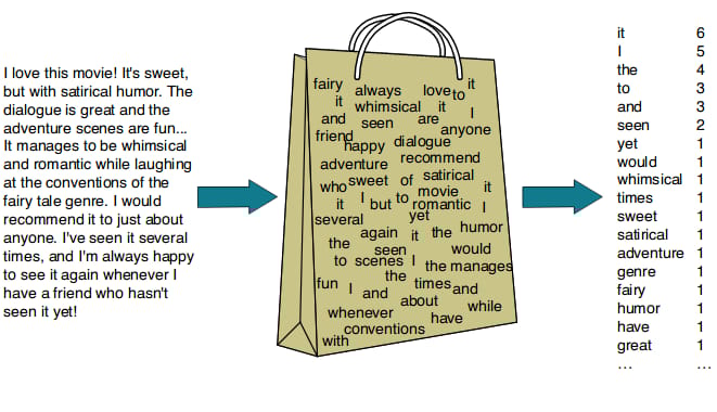
BAG OF WORD (BOW) REPRESENTATION

BOW representation doesn’t consider the position of a word in the sentences. It only considers the frequency of a word which is used to calculate all probabilities.

Now that we have addressed these, let’s build our model.

Our goal with classification is to find the class a test sentence belongs to. In other words, it is to find the class with the highest posterior probability ( P(c/s) ), which is also called the “maximum a posterior” class (C_MAP ).

To understand this better, let’s take a test sentence:

s = “the brown cat is sitting on a mat”

We will tokenize this using word-level tokenization

s = <"the","brown","cat","is","sitting","on","a","mat">

Now, the C_MAP can be written as

We want to find the class that has maximum posterior probability which is why we are using arg-max. If we substitute Bayes theorem into this equation it becomes

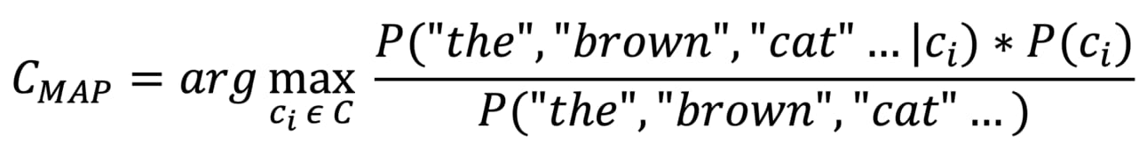
Great. But if you look at this equation carefully, you can see that the denominator is the same irrespective of the class. The evidence, which is the probability of sentence occurring across all classes) doesn’t depend on the c_i. For that reason, we can get rid of it from the equation.

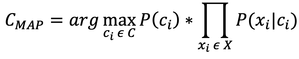
If you remember we have assumed that each word in this sentence is independent of the other. Using this assumption, we can rewrite the above equation as

This is your final equation to calculate the C_MAP. But how do you calculate the probabilities on the right side of the equation?

We will use the frequencies from the BOW representation I have defined above.

Here,

N(C = c_i) is the number of sentences in the training set that belong to class c_i.

N is the total no of sentences in the training set.

Looking at this equation should make it clear that this is constant for a class and doesn’t depend on the test sentence or any other evidence, like a prior should.

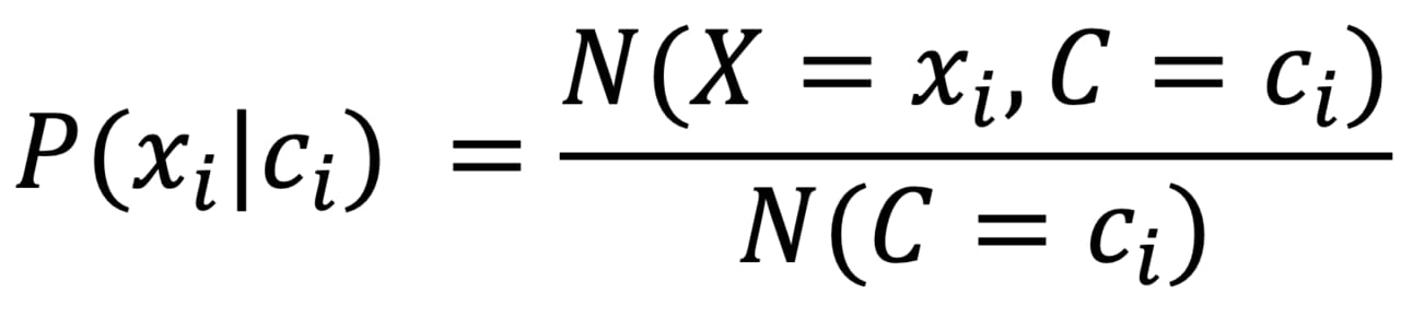
Here

N(X = ”the”, C = c_i) is the number of sentences in the training set which have the word “the” in them and belong to class c_i

You already know what N(C=c_i) is from the above equation.

This can be similarly written for any word x_i. let’s generalize this equation.

Ok. So, we have everything to calculate the posterior probability. We need to substitute these into the C_MAP equation to classify a test sentence.

That’s it, right? No. There are 2 major issues with the above equation that would make it useless in real-time scenarios. Can you guess them? (pause here and review the equations above a second time. Try to see if they break for some cases.)

1. Zero Probability

s = <"the","brown","cat","is","sitting","on","a","mat">

Let’s assume that s above is the test sentence and you are calculating the posterior for this.

You have all the equations and their calculations above. Great.

Let’s assume the word “mat” was never seen in the train set. It is an Out-Of-Vocabulary (OOV) word. What would be the likelihood of this?

It would be 0 because N(X = ”mat”, C = c_i) is 0. That is ok. Because it is not present in the train set its probability is 0.

But remember that we multiply this likelihood probability with the likelihood of other words in the sentence.

because P(“mat”|c_i) = 0, if we substitute it into the quation

Which makes C_MAP = 0. We don’t want that to happen because the probabilities of other words in the sentence are non-zero zero but they are not considered.

This would mean that if a single word in a 1000-word sentence is not seen in the train data, the probability of the entire sentence becomes 0. And OOV words are common in NLP.

So, how do you deal with this? We use smoothing techniques to assign a non-zero probability to the OOV word.

Laplace Smoothing

Laplace smoothing is the most common smoothing technique used in NLP. Here is how you change the P(X_i|c_i) equation to introduce smoothing

Where

alpha is known as a smoothing factor. It is a number between 0 to 1 where 0 removes the smoothing and 1 assigns too much probability to the OOV words. alpha is a hyper-parameter which is tuned based on validation performance

V is the vocabulary size. V is the number of unique words in training data. This is used to normalize the probabilities so that they all still add up to 1.

2. Underflow issues

Let’s assume that our test sentence has 100 words. And this particular sentence is a hard one. Most of the words in it rarely occur in train set and hence have very low probabilities.

If you remember the equation, we multiply the likelihood of one word to the other in a sentence.

And because our probabilities are so low, our posterior would be something like this

This would make the product so small that your computer would throw a floating point underflow issues. The number would have so many digits after the decimal that it cannot be stored.

In TensorFlow, this would lead to NaN errors where the product and any operation to it is converted to NaN.

How to deal with this? The problem here is the product, right? Multiplying a number less than 0 to another makes it even smaller. But that is not the case with addition. When you add two numbers less than 0, the value increases and remains in the same order as one of the numbers.

How do you convert multiplication to addition? Using Logarithms.

Our C_MAP can be generalized as follows:

And now, If we apply log to both sides of the equation

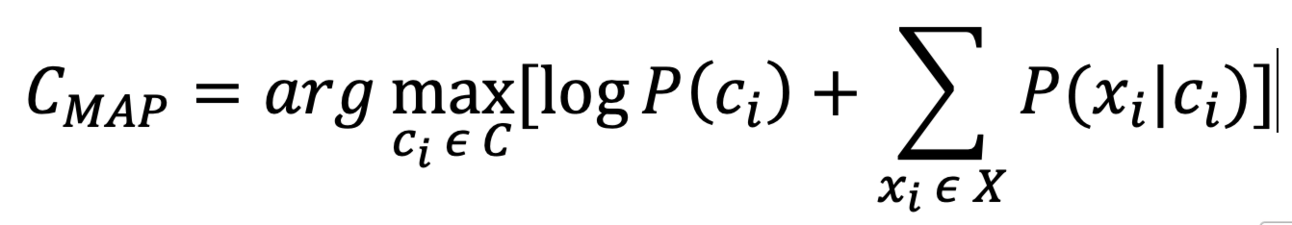
Note: Remember that the rank of the class doesn’t change when the log is applied. The class with the highest posterior probability will also have the highest log probability.

There you go. With the addition of smoothing and log to your equation, your naive Bayes classifier can be directly used for classification on real-time problems.

It most probably won’t perform well for real-time complex problems because

1. The assumptions of the naive Bayes classifier are not true in most scenarios.

2. Using only the frequency to calculate probabilities is not sophisticated. Words like “is”, ”are”, ”the” etc would dominate the probabilities as they are the most frequent words.

3. Semantic relationships are not captured as position is ignored to calculate the posterior.

Despite its simplicity, assumptions, and drawbacks, Naive Bayes Classifier is still used for spam detection and sentiment classification. It is an efficient and simple model that works great with relatively smaller data.

That’s it for this week. We will see some linear classifiers in NLP before moving to non-linear neural networks like RNNs, LSTMs, and Transformers (If you want me to directly skip to RNNs please reply to this email or leave a comment below). Thank you.